Financial literacy in schools, hurray!

We need as many friends as we can get when investing, right? And adding some bonds to an investment portfolio helps reduce the volatility when share markets head south, so to speak. Shares go down in a crisis, and bonds go up, to help balance out the returns, is how traditional portfolio design works.
Not so, for the regular saver, contributing a percentage of their income every month for their retirement into a KiwiSaver portfolio. This process of regular saving into a volatile investment portfolio has a name, dollar-cost averaging.
Dollar cost averaging harnesses volatility turning it into a tool rather than a weapon for the long-term regular saver.
This visual below illustrates two different portfolios. Portfolio A (red line, a “hare”) is a portfolio containing volatile shares and portfolio B (grey line, a “tortoise”) is a more defensive cash and fixed interest (bonds) portfolio with no volatility.
For this example, both portfolios start and finish at the same unit price. We are not assuming that the share portfolio earns any more than the bond portfolio. In reality, the share portfolio will most likely earn a lot more than the defensive portfolio over the long term, but we are not wanting to show that here. We are just looking at how volatility can work to the saver’s advantage without addressing the higher return from shares over the long term. Let’s leave that for later.
Both portfolios begin at $0 in 2020 with their unit prices being $5 each. During our six-year period, the owners of both portfolios put in $1,000 per month. At the end of 2026, each portfolio’s unit price is a matching $11.
Portfolio A, the hare, has gyrated around going to $8 in the first year, then falling to $4 a unit by the end of the second year. Portfolio B, the tortoise, is marching steadily on. It is a much more comfortable ride being a tortoise than it is being a hare. But who is better off, the tortoise, or the hare by the end of the period? Have a look at the graph and the underlying tables.
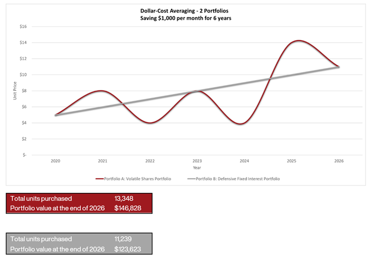
You would think that given both portfolios started and finished at the same unit value, by 2026 they would contain the same amount of money in each portfolio … right? Not quite.
Portfolio A ends up with $23,000 more than portfolio B! With regular saving over the long term, it pays to back the hare rather than the tortoise. Volatility is a friend to the regular saver.
This is where the magician pulls the rabbit out of her hat and explains her “magic.”
How is the ending balance different when they invest the same amount each month, started and stopped at the same unit price? Well, it is the work being done by volatility. Cash flow is important and for the technically minded, it is the difference between the internal rate of return (IRR) and time-weighted return. The time-weighted return is the return on the first dollar being invested and both portfolios have the same time-weighted return. But due to the cash flows being at different prices, the portfolios have a different IRR.
When portfolio A’s unit price goes up, you buy less units than portfolio B. But when the unit price drops to $4, portfolio A buy a lot more units (250) than portfolio B (167).
In our example, portfolio A has 2,000 more units in it than portfolio B by the end of the period.
Since you accumulate more shares when the market is down below the value of the steady portfolio B, your portfolio is worth more when it recovers back to $11.
Of course, the positive impact of dollar-cost averaging depends upon the unit price spending some time below the average price. It wouldn’t work if portfolio A spent all that time above portfolio B until the last minute and then fell to $11. In that case portfolio B would be better than portfolio A.
In this example we used a timeline of only six years. A relatively short period to hold investments as a serious long-term investor. Even in such a short period you can see the potential of dollar cost averaging at work, so long as you get some serious volatility downwards. If you extrapolate this concept over an investment timeline of say 20 or 30 years with some decent market crashes thrown in, the difference in the end results could compound into a very large difference in value.
Combine this with another wonder of the investment world - shares most likely out-perform cash and fixed interest over the long term, then you’ve really got a recipe for success.
If, in the example above the defensive portfolio B didn’t match the end value of portfolio A; it ended up at $7 per unit rather than the portfolio A unit price of $11? In other words, portfolio A out-performed portfolio B. Portfolio A is still worth $146,828, whereas portfolio B is now worth $83,033, or $63,794 less than portfolio A. This is more like real life over the long term.
Regular savers should start celebrating whenever the markets fall, allowing them to mop up cheap assets with their monthly savings.
It pays to work out who your friends are!
Keep asking great questions…

P.S. This article does not constitute personal financial advice. As with all things financial, get some good personal financial planning advice before choosing your KiwiSaver fund. Everyone has a different set of risks.